Normalizing Flows for Sampling-Based Motion Planning

This project was developed as part of the PhD course in Advanced Topics on Robotics.

Introduction

Sampling-based motion planning (SBMP) is a popular approach for solving robotic motion planning problems. In most cases, the objective is to find a trajectory from an initial state to a target state, while complying with kinematic constraints or avoiding collisions. Most SBMP algorithms build a graph, starting from the initial state, and iteratively sample new candidate states that add to the graph until the target state is found. Traditional methods uniformly sample the configuration space for new candidate states. This is inefficient, especially in high dimensions as the volume of the configuration space grows exponentially with the number of degrees of freedom.

Recently, learning-based samplers have been proposed that integrate additional information about the problem, such as demonstrations, identified critical states, or past solved problems (Ichter et al. 2017, Lai et al. 2020, Shah et al. 2020). Using this information a new sampling function can be learned that proposes states that can avoid obstacles or be closer to critical regions of the configuration space. To learn the new sampling function from data generative models can have been employed such as Variational Autoencoders or Flow-based models. Learning-based samplers have been shown to outperform traditional uniform samplers in solving times, optimal cost, success rates, and number of samples used.

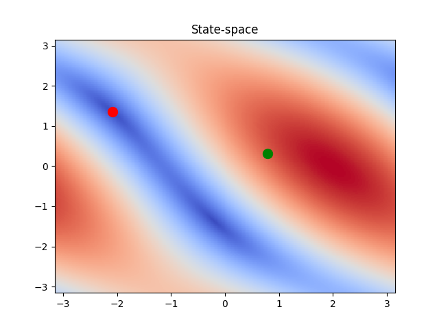
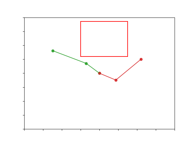
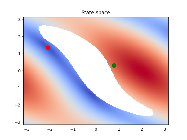
Let's consider the problem of planning a trajectory for the 2DoF robotic manipulator, shown in the right figure below, to reach a target (green) state from the initial (red) state. In the left figure, we see the 2D state space of the manipulator. The colormap denotes the distance of each state, to the target state.

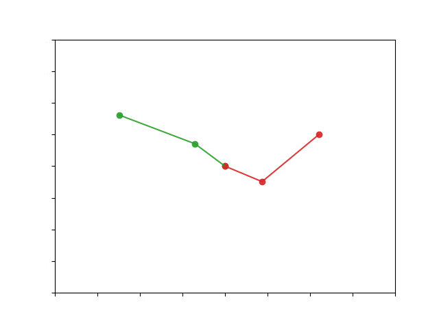
In this simple case, linearly interpolating between the two states would produce a smooth trajectory that moves the manipulator to the desired position. The trajectory in the configuration and the state space is shown below.

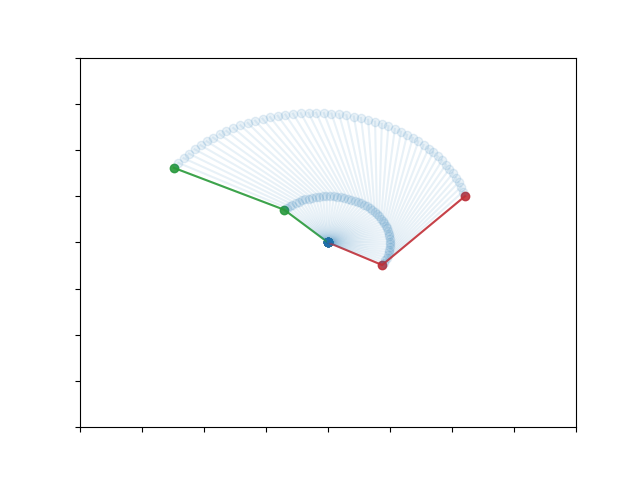
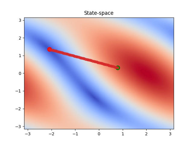
If we add an obstacle (red box) in the workspace then this solution is no longer possible as the manipulator is going to collide with the obstacle. This is better seen if we transfer the problem to the state space of the system. We can see that the obstacle creates a "hole" in the state space (white region) that the manipulator is in collision with the obstacle. The problem then is to find a trajectory from the initial state to the target one, while avoiding the region of invalid states. This is a classic problem for sampling-based motion planners.

Background

Rapidly-exploring Random Tree (RRT)

We use the Rapidly-exploring Random Tree (RRT) algorithm as our baseline. RRT is one of the most simple SBMP algorithms. It starts from the initial state and repeatedly samples new candidate states, if these states are not in collision with the environment, they are added to the tree. The algorithm terminates when the target state is encountered in a neighborhood near one of the leaves. Then a path is computed by backtracking to the initial state. Usually, the new candidate states are sampled from a uniform distribution.

RRT_UNIFORM( $S, s_0, s_{target}, C$ )
     initialize graph $G$
     initialize $goal\_found = False$
     while not $goal\_found$
          sample uniform random state $s_{rand} \in S$
          find nearest vertex $s_{near} \in G$
          get new state $s_{new}$
          check for collisions
          if no collisions found: $G.add\_vertex(s_{new})$
          if $s_{new} == s_{target}$: backtrack to $s_0$.
     return $path$.

Normalizing Flows

Normalizing flows is a framework to approximate complex distributions and generate new samples. The main idea behind it is that if we have a distribution $\mathbf{u} \sim p_{\mathrm{u}}(\mathbf{u})$ that is easy to sample from, and a series of transformations $\mathbf{x}=T_i(\mathbf{u})$ we can transform the initial distribution to an arbitrary distribution. If these transformations are invertible and differentiable, then for each sample in our dataset we can exactly compute its likelihood as: $$ p_{\mathbf{x}}(\mathbf{x})=p_{\mathbf{u}} (\mathbf{u})\left|\operatorname{det} J_{T} (\mathbf{u})\right|^{-1} \quad \text { where } \mathbf{u}=T^{-1}(\mathbf{x}) $$ This allows us to easily train our model using maximum likelihood estimation. The main bottleneck in the computation of the MLE objective is the calculation of the inverse determinant of the Jacobian of the transformation. So, a common approach is to choose transformations that have a structure which facilitates this computation. For example, transforms whose Jacobian is triangular, so the computation of the determinant is the product of the diagonal elements. The transforms $T_i$ can be represented by neural networks and then we can train the networks using standard gradient descent optimizers. For a more in-depth introduction to normalizing flows check this paper and this blog post.

Case Study

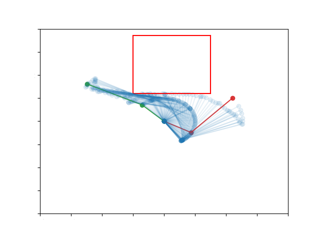
If we apply the RRT algorithm to the toy problem described before it will start creating a tree like structure around the initial state until it reaches the target one. Then it will create a path backwards to the initial state. The solution in the configuration and state space is shown below.

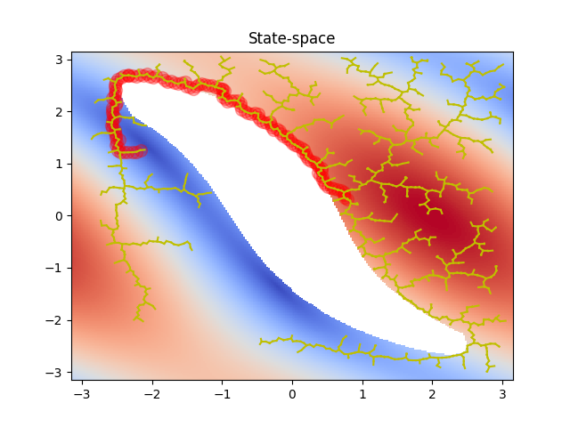
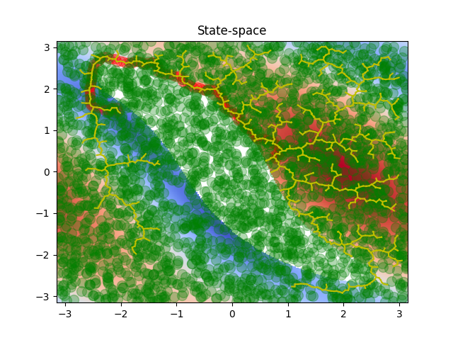
However, uniformly sampling candidate states is inefficient, since a lot of the possible states can be invalid due to collisions. In addition, no information about the workspace is taken into account, such as possible critical states. Below are shown all the states that RRT examined in order to solve the problem. We can see that a lot of these states are invalid.

In order to improve this inefficiency, we can learn a new sampling function that is specific to this environment. We will use the Masked Autoregressive Flow transform (Papamakarios et al. 2017) to estimate the new density. Mathematically, the transform is given by $$ x_{i}=u_{i} \exp (\alpha_{i})+\mu_{i} $$ $$\text { where } \mu_{i}=f_{\mu_{i}}\left(\mathbf{x}_{1: i-1}\right), \quad \alpha_{i}=f_{\alpha_{i}}\left(\mathbf{x}_{1: i-1}\right) $$ $$\text { and } u_{i} \sim \mathcal{N}(0,1)$$ In this case, the easy to sample distribution is the standard normal distribution $\mathcal{N}(0,1)$, $x$ is the transformed variable whose each component $x_i$ is a function of the previous components $\mathbf{x}_{1: i-1}$, hence the autoregressive part. Finally, the functions $f_{\mu_{i}}, f_{\alpha_{i}}$ are implemented with neural networks. The Jacobian of this transform is triangular so it can be computed efficiently.

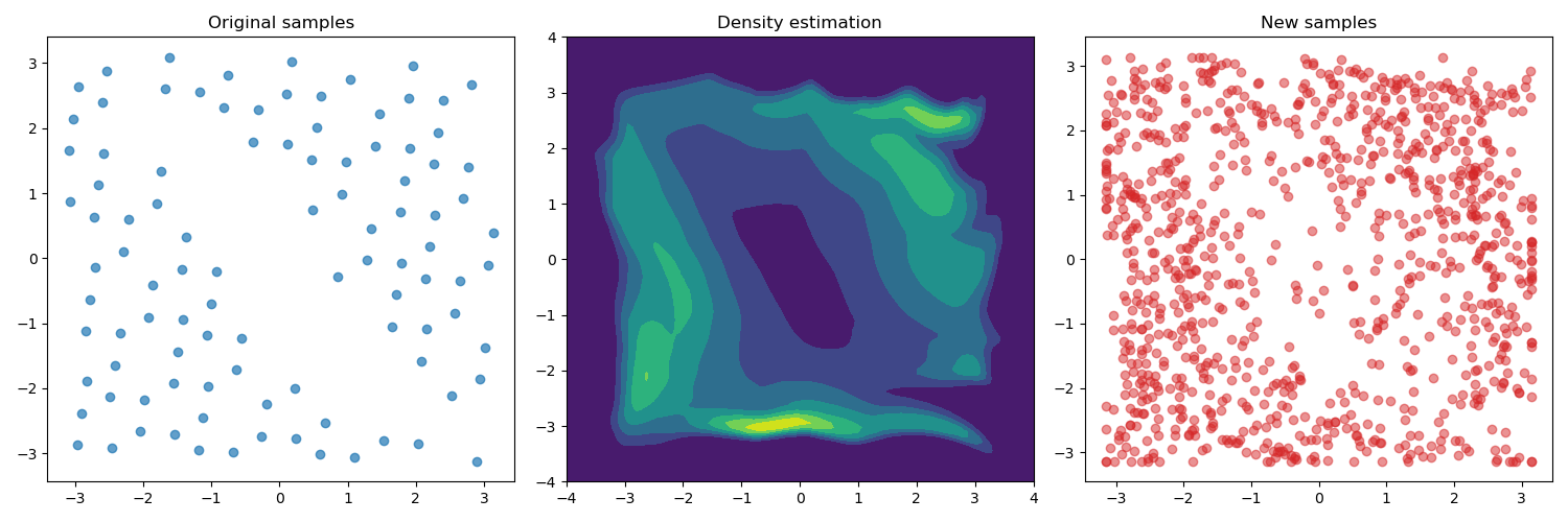
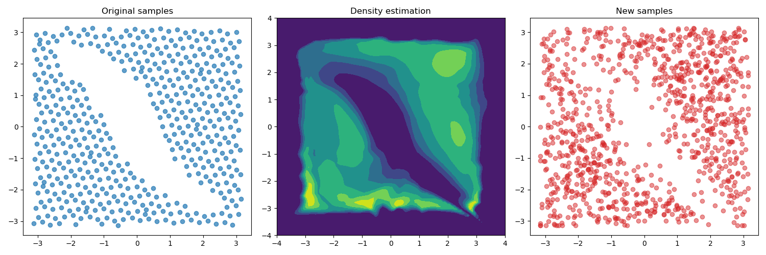
The question now is on what data we will train our model. The simplest one is probably to just uniformly sample the configuration space, determine if each state is valid, i.e. not in collision, and use the valid states as the training dataset. The result of this approach for our toy problem is shown in the figures below. The figures on the right show the valid sampled states from the configuration space. We used a low discrepancy quasi-random sequence to get samples that cover the entire space. The upper figure has $100$ samples and the lower $500$ samples. The middle figures show the density estimated from the model. Both densities exhibit a "hole" in the center where the obstacle lies. Finally, the left figures show new states samples from the estimated densities. The new samples tend to not be in the invalid region of the state space.

Various alternative methods exist for selecting the training data. One approach is to collect a set of demonstrations and use the paths as training data. For instance, we can solve some initial random path planning problems using the baseline RRT algorithm, and compile a dataset with the states from the demonstrations. Another option is to train the density estimation method on the ”critical” states of the environment, i.e. the states that are encountered in most demonstrations.

The figures below show the outcomes of training the model on three different datasets collected using the approaches mentioned before. For this case, we added one more obstacle in the environment, which corresponds to the additional "hole" in the state space. The first row shows the results obtained from the uniformly sampled data, while the second row shows the demonstrations collected by solving a set of path planning problems using the RRT algorithm. Finally, the third row shows the "critical states" extracted from the problems. In this case, the "critical states" were defined a the middle states of the paths.

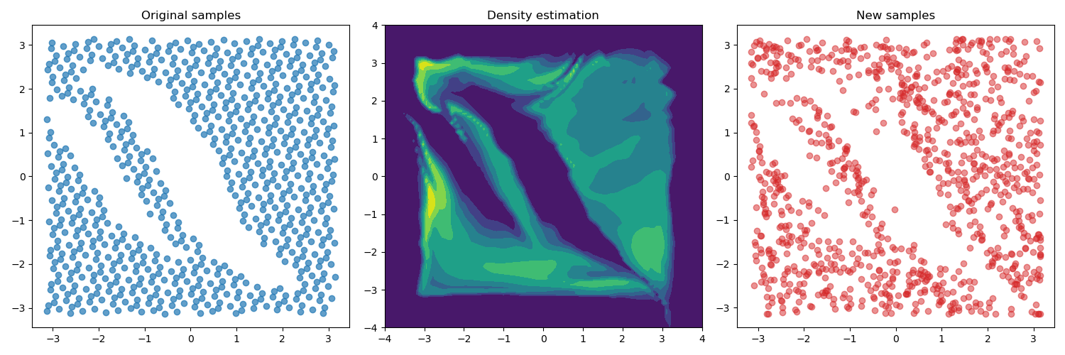
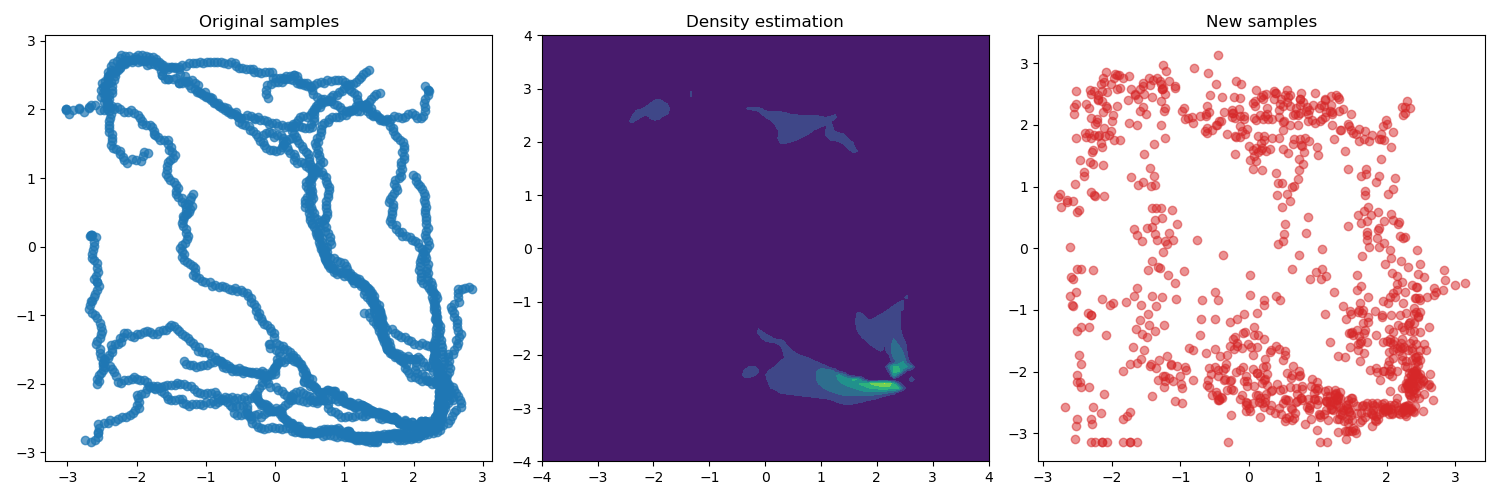
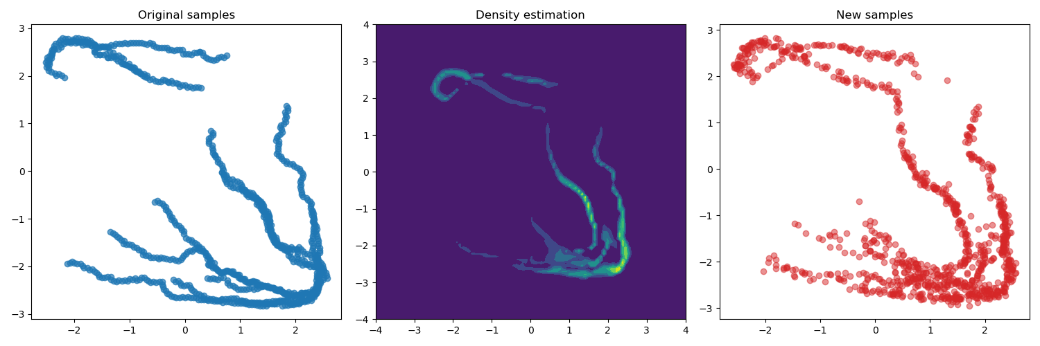
As we can see from the results above the flow model is able to estimate accurately the provided data and generate new samples accordingly. But we can notice that the models trained using data from demonstrations and critical states tend to generate samples that do not adequately cover the entire state space. Consequently, if the target state lies outside the scope of the demonstrations, it becomes unlikely that the algorithm will explore these regions. To address this in practice, we use a mixture of the flow based sampler and the uniform sampler. Specifically, in each iteration we sample the new state from the flow sampler with probability $λ$ and from the uniform sampler with probability $1 − λ$. This approach ensures that we sample states from the entirety of the state space while also maintaining a clustering of states in regions covered by the training data. Finally, another practical factor to take into account is that sampling from the flow model is significantly more computationally expensive compared to sampling from a uniform distribution. To mitigate this, we can use a batch sampling approach, where we sample a batch of N states, process them, and if the target is not found, we proceed to sample a new batch.

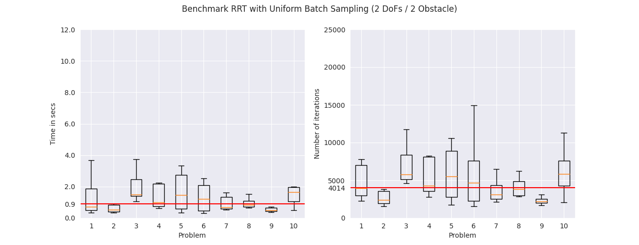
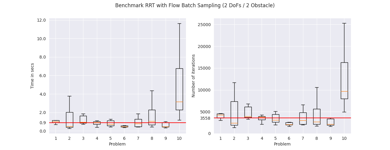
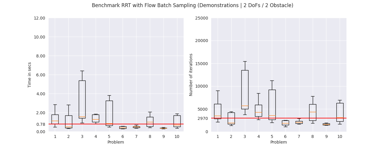
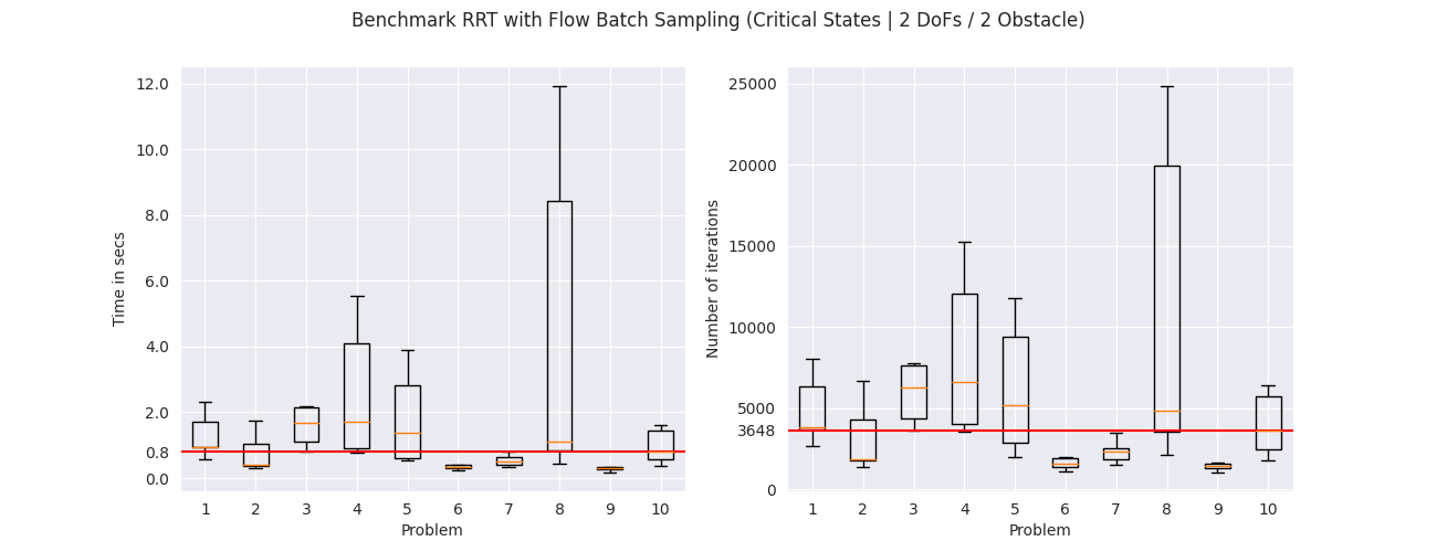
To evaluate the different sampling strategies we applied them on $10$ random problems. Each problem was solved $10$ times with different seeds. The figures below show the total execution time to solve each problem and the number of iterations in a box plot format. The box in the plot represents the interquartile range, meaning the range from the first quartile to the third quartile. The orange line in the middle shows the median of the values. The median among all problems is shown with the red line. From the results we get that the RRT with the uniform sampler is slower, in the median case, compared to the RRT with the flow sampler trained on uniformly sampled states. The RRT with the flow sampler trained on demonstrations and critical states further improve the median running time for all environments. The same pattern can be seen in the number of iterations that are needed for each problem, where the flow samplers trained on demonstrations and critical states need less samples compared to the flow sampler trained on uniformly sampled states and the uniform sampler. These results suggest that learning-based samplers can potentially improve the execution times of sampling-based motion planning algorithms.

Conclusion

We saw an alternative to the traditional uniform sampler used in sampling-based motion planning algorithms. This learning-based sampler, uses normalizing flow neural networks to estimate new distributions that can be used to sample from. This distribution encodes information about the environment such as the position of obstacles, already seen paths, and critical states. We saw that by using this distribution to sample states we can improve the execution time of the planning algorithm and the number of samples needed. On the other hand, this type of sampler cannot be used in dynamic environments, for example where there might be people moving around. An interesting future research direction would be to design conditional samplers that can take the position of the obstacle as input.

References

[1] Ichter et al. “Learning Sampling Distributions for Robot Motion Planning.” ICRA, 2017.

[2] Shah et al. “Learning and Using Abstractions for Robot Planning.” ArXiv, 2020.

[3] Lai et al. “Learning to Plan Optimally with Flow-based Motion Planner.” ArXiv, 2020.

[4] Papamakarios et al. “Masked Autoregressive Flow for Density Estimation.” ArXiv, 2017.